Probability Distributions
Probability distributions describe how the values of a random variable are distributed. Different types of probability distributions are used based on the nature of the data and the problem being analyzed.
Binomial Distribution
Description
The Binomial distribution represents the number of successes in a fixed number of independent trials, each with the same probability of success. It is used when there are two possible outcomes: success or failure.
Formula
P(X=k) = (nCk) * pk * (1−p)n−k
- n = number of trials
- k = number of successes
- p = probability of success
- nCk = combinations formula
Example Use Cases
- The number of heads obtained when flipping a fair coin 10 times.
- The number of defective items in a batch of 50 products.
Binomial Distribution Chart (n=10, p=0.5)
    import numpy as np
    import matplotlib.pyplot as plt
    import scipy.stats as stats

    # Parameters for Binomial Distribution
    n = 10  # Number of trials
    p = 0.5  # Probability of success

    # Generate Binomial distribution probabilities
    x = np.arange(0, n+1)
    binom_pmf = stats.binom.pmf(x, n, p)

    # Plot Binomial Distribution
    plt.figure(figsize=(8,5))
    plt.bar(x, binom_pmf, color='blue', alpha=0.7, edgecolor='black')
    plt.xlabel('Number of Successes (k)')
    plt.ylabel('Probability')
    plt.title(f'Binomial Distribution (n={n}, p={p})')
    plt.xticks(x)
    plt.grid(axis='y', linestyle='--', alpha=0.7)
    plt.show()

Normal Distribution
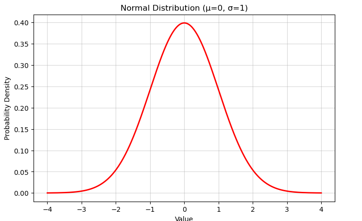
The Normal distribution is a continuous probability distribution that is symmetric around the mean, describing many natural phenomena such as heights, test scores, and measurement errors.
    # Parameters for Normal Distribution
    mu = 0   # Mean
    sigma = 1  # Standard Deviation

    # Generate Normal distribution values
    x = np.linspace(mu - 4*sigma, mu + 4*sigma, 1000)
    normal_pdf = stats.norm.pdf(x, mu, sigma)

    # Plot Normal Distribution
    plt.figure(figsize=(8,5))
    plt.plot(x, normal_pdf, color='red', lw=2)
    plt.xlabel('Value')
    plt.ylabel('Probability Density')
    plt.title(f'Normal Distribution (μ={mu}, σ={sigma})')
    plt.grid(alpha=0.5)
    plt.show()

t-Distribution
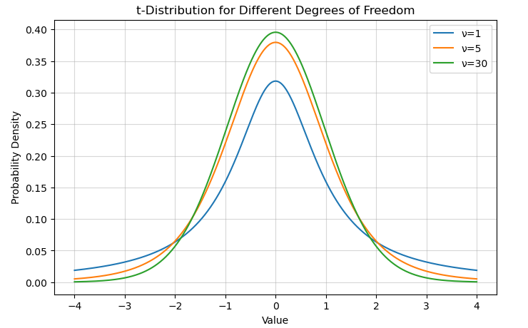
The t-distribution is similar to the normal distribution but has heavier tails. It is used in statistics for small sample sizes when estimating population parameters.
    # Parameters for t-Distribution
    df_values = [1, 5, 30]  # Different degrees of freedom

    # Generate t-distribution values
    x = np.linspace(-4, 4, 1000)

    # Plot t-Distribution for different degrees of freedom
    plt.figure(figsize=(8,5))
    for df in df_values:
    t_pdf = stats.t.pdf(x, df)
    plt.plot(x, t_pdf, label=f'ν={df}')

    plt.xlabel('Value')
    plt.ylabel('Probability Density')
    plt.title('t-Distribution for Different Degrees of Freedom')
    plt.legend()
    plt.grid(alpha=0.5)
    plt.show()

Chi-Squared Distribution
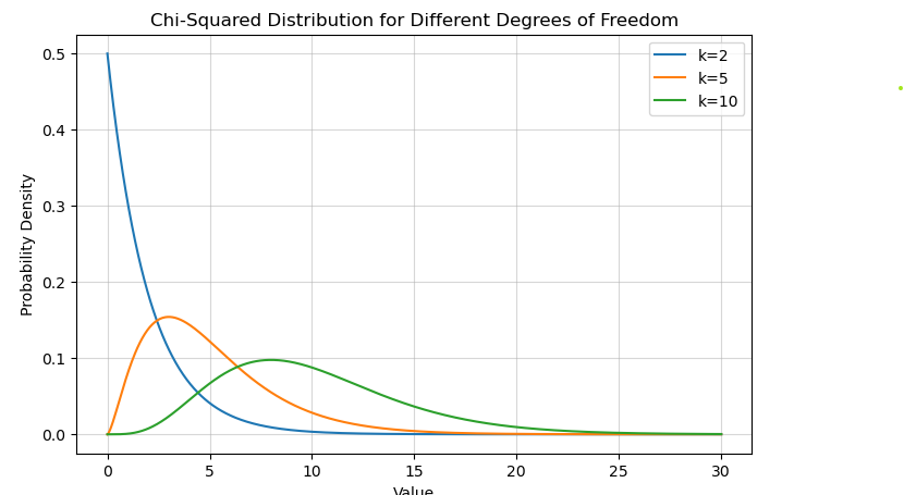
The Chi-squared distribution is used in hypothesis testing, especially in tests of independence and goodness of fit.
    # Parameters for Chi-Squared Distribution
    df_values = [2, 5, 10]  # Different degrees of freedom

    # Generate Chi-Squared distribution values
    x = np.linspace(0, 30, 1000)

    # Plot Chi-Squared Distribution
    plt.figure(figsize=(8,5))
    for df in df_values:
    chi2_pdf = stats.chi2.pdf(x, df)
    plt.plot(x, chi2_pdf, label=f'k={df}')

    plt.xlabel('Value')
    plt.ylabel('Probability Density')
    plt.title('Chi-Squared Distribution for Different Degrees of Freedom')
    plt.legend()
    plt.grid(alpha=0.5)
    plt.show()

F-Distribution
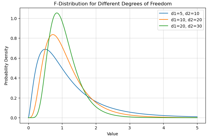
The F-distribution is commonly used in ANOVA (Analysis of Variance) to compare variances between groups.
    # Parameters for F-Distribution
    df_pairs = [(5, 10), (10, 20), (20, 30)]  # Different (d1, d2) values

    # Generate F-distribution values
    x = np.linspace(0, 5, 1000)

    # Plot F-Distribution
    plt.figure(figsize=(8,5))
    for d1, d2 in df_pairs:
    f_pdf = stats.f.pdf(x, d1, d2)
    plt.plot(x, f_pdf, label=f'd1={d1}, d2={d2}')

    plt.xlabel('Value')
    plt.ylabel('Probability Density')
    plt.title('F-Distribution for Different Degrees of Freedom')
    plt.legend()
    plt.grid(alpha=0.5)
    plt.show()

Summary of Statistical Distributions
| Distribution | Used For | Key Feature |
|---|---|---|
| Binomial | Success/failure outcomes in trials | Discrete, depends on number of trials and probability |
| Normal | Natural phenomena like heights, test scores | Continuous, symmetric bell curve |
| t-Distribution | Small-sample hypothesis testing | Similar to normal but with heavier tails |
| Chi-Squared | Hypothesis testing for categorical data | Right-skewed, sum of squared normal variables |
| F-Distribution | Comparing two variances (ANOVA) | Right-skewed, depends on two degrees of freedom |
Each of these distributions plays a crucial role in statistics, data science, and hypothesis testing. Let me know if you need more details! 🚀